Setup:
Use the file traffic_accidents.csv for your analysis. The column names are:
Variable Description
accidents Number of recorded accidents, as a positive integer.
traffic_fine_amount Traffic fine amount, expressed in thousands of USD.
traffic_density Traffic density index, scale from 0 (low) to 10 (high).
traffic_lights Proportion of traffic lights in the area (0 to 1).
pavement_quality Pavement quality, scale from 0 (very poor) to 5 (excellent).
urban_area Urban area (1) or rural area (0), as an integer.
average_speed Average speed of vehicles in km/h.
rain_intensity Rain intensity, scale from 0 (no rain) to 3 (heavy rain).
vehicle_count Estimated number of vehicles, in thousands, as an integer.
time_of_day Time of day in 24-hour format (0 to 24).
accidents traffic_fine_amount
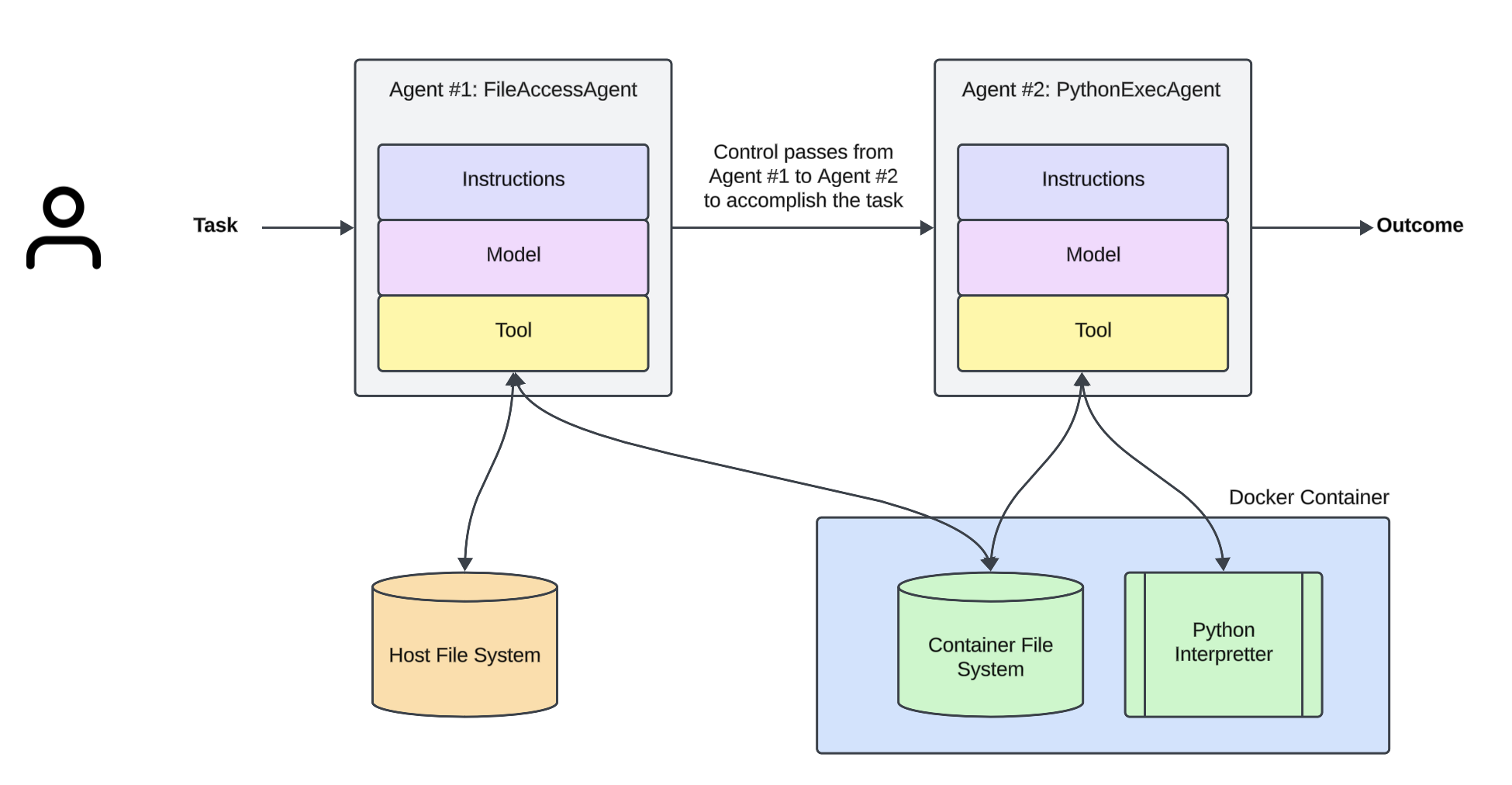
Setting up the agents...
Understanding the contents of the file...
2025-02-03 13:03:54,066 - MyApp - INFO - Handling tool call: safe_file_access
2025-02-03 13:03:54,067 - MyApp - INFO - Tool arguments: {'filename': './resources/data/traffic_accidents.csv'}
2025-02-03 13:03:54,562 - MyApp - INFO - Tool 'safe_file_access' response: Copied ./resources/data/traffic_accidents.csv into sandbox:/home/sandboxuser/.
The file content for the first 15 rows is:
    accidents  traffic_fine_amount  traffic_density  traffic_lights  pavement_quality  urban_area  average_speed  rain_intensity  vehicle_count  time_of_day
0          20               4.3709           2.3049         753.000            0.7700           1        321.592          1.1944       290.8570     160.4320
1          11               9.5564           3.2757           5.452            4.0540           1        478.623          6.2960       931.8120       8.9108
2          19               7.5879           2.0989           6.697          345.0000           0        364.476          2.8584       830.0860       5.5727
3          23               6.3879           4.9188           9.412            4.7290           0         20.920          2.1065       813.1590     131.4520
4          23               2.4042           1.9610           7.393            1.7111           1         37.378          1.7028         1.4663       6.9610
5          31               2.4040           6.7137           5.411            5.9050           1        404.621          1.8936       689.0410       8.1801
6          29               1.5228           5.2316           9.326            2.3785           1         16.292          2.5213       237.9710      12.6622
7          18               8.7956           8.9864           4.784            1.9984           0        352.566          1.9072       968.0670       8.0602
8          15               6.4100           1.6439           5.612            3.6090           1        217.198          3.4380       535.4440       8.2904
9          22               7.3727           8.0411           5.961            4.7650           1        409.261          2.0919       569.0560     203.5910
10         28               1.1853           7.9196           0.410            3.7678           1        147.689          1.6946       362.9180     224.1580
11         17               9.7292           1.2718           8.385            8.9720           0         46.888          2.8990       541.3630     198.5740
12         14               8.4920           3.9856           1.852            4.6776           0        287.393          2.2012        75.2240       2.3728
13         21               2.9111           1.7015           5.548            1.9607           1        176.652          1.0320       566.3010       6.9538
14         22               2.6364           2.5472           7.222            2.3709           0        209.686          4.0620        64.4850     170.7110
Type your question related to the data in the file. Type 'exit' to exit.
User question: What factors contribute the most to accident frequency?
Generating dynamic tools and using code interpreter...
2025-02-03 13:04:39,427 - MyApp - INFO - Handling tool call: execute_python_code
2025-02-03 13:04:39,429 - MyApp - INFO - Tool arguments: {'python_code': "import pandas as pd\nimport numpy as np\nfrom sklearn.linear_model import LinearRegression\nfrom sklearn.preprocessing import StandardScaler\nimport matplotlib.pyplot as plt\nimport seaborn as sns\n\n# Load the dataset\nfile_path = '/home/sandboxuser/traffic_accidents.csv'\ndf = pd.read_csv(file_path)\n\n# Show basic information\nprint('Dataset shape:', df.shape)\nprint('First few rows:')\nprint(df.head(), '\\n')\nprint('Columns:', df.columns.tolist(), '\\n')\n\n# Correlation matrix analysis\ncorr_matrix = df.corr()\nprint('Correlation matrix:')\nprint(corr_matrix, '\\n')\n\n# Correlation of each feature with accidents\nacc_corr = corr_matrix['accidents'].drop('accidents').sort_values(key=lambda x: abs(x), ascending=False)\nprint('Correlation of other variables with accidents (sorted by absolute correlation):')\nprint(acc_corr, '\\n')\n\n# Visualize the correlation matrix\nplt.figure(figsize=(10, 8))\nsns.heatmap(corr_matrix, annot=True, cmap='coolwarm', fmt='.2f')\nplt.title('Correlation Matrix')\nplt.tight_layout()\nplt.savefig('correlation_matrix.png')\nplt.close()\n\n# Prepare data for regression analysis\n# Exclude target variable 'accidents'\nfeatures = [col for col in df.columns if col != 'accidents']\nX = df[features]\ny = df['accidents']\n\n# Standardize the features to compare the regression coefficients on the same scale\nscaler = StandardScaler()\nX_scaled = scaler.fit_transform(X)\n\n# Fit a linear regression model\nmodel = LinearRegression()\nmodel.fit(X_scaled, y)\n\n# Gather coefficients along with feature names\ncoef = model.coef_\ncoef_df = pd.DataFrame({'Feature': features, 'Coefficient': coef})\ncoef_df['AbsCoefficient'] = coef_df['Coefficient'].abs()\ncoef_df = coef_df.sort_values(by='AbsCoefficient', ascending=False)\nprint('Linear Regression Coefficients (using standardized features):')\nprint(coef_df[['Feature', 'Coefficient']], '\\n')\n\n# Additionally, compute feature importances using a Random Forest regressor\nfrom sklearn.ensemble import RandomForestRegressor\nrf = RandomForestRegressor(random_state=42)\nrf.fit(X, y)\nrf_importance = rf.feature_importances_\nrf_df = pd.DataFrame({'Feature': features, 'Importance': rf_importance})\nrf_df = rf_df.sort_values(by='Importance', ascending=False)\nprint('Random Forest Feature Importances:')\nprint(rf_df, '\\n')\n\n# The printed outputs will help in understanding which factors contribute most to accident frequency.\n\n# For clarity, save the coefficients and importances to CSV files (optional)\ncoef_df.to_csv('linear_regression_coefficients.csv', index=False)\nrf_df.to_csv('random_forest_importances.csv', index=False)\n\n# End of analysis\n"}
2025-02-03 13:04:43,123 - MyApp - INFO - Tool 'execute_python_code' response: Dataset shape: (8756, 10)
First few rows:
   accidents  traffic_fine_amount  ...  vehicle_count  time_of_day
0         20               4.3709  ...       290.8570     160.4320
1         11               9.5564  ...       931.8120       8.9108
2         19               7.5879  ...       830.0860       5.5727
3         23               6.3879  ...       813.1590     131.4520
4         23               2.4042  ...         1.4663       6.9610

[5 rows x 10 columns]

Columns: ['accidents', 'traffic_fine_amount', 'traffic_density', 'traffic_lights', 'pavement_quality', 'urban_area', 'average_speed', 'rain_intensity', 'vehicle_count', 'time_of_day']

Correlation matrix:
                     accidents  traffic_fine_amount  ...  vehicle_count  time_of_day
accidents             1.000000            -0.745161  ...       0.068399     0.101995
traffic_fine_amount  -0.745161             1.000000  ...      -0.016610    -0.006236
traffic_density      -0.059265            -0.004365  ...      -0.014244     0.002806
traffic_lights       -0.026642             0.009056  ...       0.001373    -0.001971
pavement_quality      0.064694            -0.021229  ...       0.007840     0.000055
urban_area            0.145092            -0.005136  ...      -0.006053    -0.006320
average_speed         0.093923             0.009151  ...       0.000777    -0.005338
rain_intensity       -0.091673            -0.015302  ...      -0.025933    -0.013446
vehicle_count         0.068399            -0.016610  ...       1.000000    -0.009303
time_of_day           0.101995            -0.006236  ...      -0.009303     1.000000

[10 rows x 10 columns]

Correlation of other variables with accidents (sorted by absolute correlation):
traffic_fine_amount   -0.745161
urban_area             0.145092
time_of_day            0.101995
average_speed          0.093923
rain_intensity        -0.091673
vehicle_count          0.068399
pavement_quality       0.064694
traffic_density       -0.059265
traffic_lights        -0.026642
Name: accidents, dtype: float64

Linear Regression Coefficients (using standardized features):
               Feature  Coefficient
0  traffic_fine_amount    -3.891935
4           urban_area     0.739618
5        average_speed     0.533698
6       rain_intensity    -0.532251
8          time_of_day     0.512661
1      traffic_density    -0.331997
7        vehicle_count     0.281283
3     pavement_quality     0.264987
2       traffic_lights    -0.092800

Random Forest Feature Importances:
               Feature  Importance
0  traffic_fine_amount    0.580838
1      traffic_density    0.165201
6       rain_intensity    0.095124
8          time_of_day    0.035814
5        average_speed    0.035590
3     pavement_quality    0.032177
2       traffic_lights    0.022613
7        vehicle_count    0.021006
4           urban_area    0.011637
Output...
The analysis shows that one variable stands out by far:

• Both the simple correlation analysis and regression results indicate that traffic_fine_amount is the dominant factor—its correlation with accidents is strong (about –0.75), and in the standardized linear regression its coefficient is the largest in magnitude (around –3.89). The negative sign suggests that, in this data, higher fine amounts are associated with fewer accidents (which might reflect more stringent enforcement or deterrence).

Other findings include:

• The Random Forest model also ranks traffic_fine_amount as most important (importance ≈ 0.58), with the next most influential factor being traffic_density (importance ≈ 0.17). Although its simple correlation with accidents is lower, traffic_density may contribute non‐linearly.

• Additional factors like urban_area, average_speed, rain_intensity, and time_of_day have moderate associations (with linear model coefficients ranging between about ±0.5 to +0.74). These suggest that accidents tend to be somewhat higher in urban areas and vary with time of day and weather conditions, but their overall impact is much less than that of traffic fine amounts.

In summary, the data analysis indicates that traffic_fine_amount contributes the most to accident frequency—with higher fines linked to fewer recorded accidents—while factors such as traffic density, urban area status, vehicle speed, rain intensity, and time of day also play secondary roles.
Type your question related to the data in the file. Type 'exit' to exit.
Exiting the application.